Hands-on: Detecting forest disturbance through time - CEF 2026

Forest disturbance changes canopy structure, vegetation moisture, and spectral reflectance. In this activity, you will use annual Landsat NBR to detect canopy disturbance from 2000 to 2025.

The workflow starts at the pixel level. You will first inspect how NBR changes through time for a selected pixel, then scale the same logic to the full ROI.

Learning objectives¶

By the end of this activity, you should be able to:

load Landsat 5, 7, 8, and 9 Surface Reflectance data
harmonize bands across Landsat sensors
mask cloud, cloud shadow, snow, and saturated pixels
calculate annual summer NBR composites
calculate year-to-year NBR drop
inspect NBR and disturbance time series for a clicked pixel
map the strongest disturbance year across the ROI
estimate disturbed area by year
export final disturbance maps
publish a GEE app

Why Landsat?¶

Sentinel-2 is useful for recent, high-resolution vegetation monitoring, but it does not cover the full 2000 to 2025 period. Landsat provides the long historical record needed for multidecadal forest disturbance analysis.

In this activity, Landsat 5, 7, 8, and 9 are combined into one harmonized image collection.

Concept¶

The Normalized Burn Ratio, or NBR, is often used to detect forest disturbance because it responds strongly to changes in canopy cover, vegetation moisture, and exposed soil.

NBR = (NIR - SWIR2) / (NIR + SWIR2)

Dense, moist forest usually has high NBR. Harvested, burned, or otherwise disturbed areas usually have lower NBR.

In this activity, disturbance is calculated as a year-to-year drop in NBR:

Disturbance = previous year NBR - current year NBR

Large positive values indicate canopy loss.

For example:

NBR in 2018 = 0.70
NBR in 2019 = 0.35

Disturbance = 0.70 - 0.35 = 0.35

A disturbance value of 0.35 indicates a strong NBR drop between 2018 and 2019.

Important interpretation note¶

This workflow detects spectral canopy disturbance. It does not directly identify the cause of disturbance.

A strong NBR drop may indicate harvesting, but it may also result from fire, windthrow, insect damage, road construction, flooding, residual clouds, cloud shadows, or other land-cover changes.

For this reason, the final map should be interpreted as forest disturbance or likely harvesting only after validation with independent information.

Complete GEE script¶

Copy the script below into the Google Earth Engine Code Editor.

// ------------------------------------------------------------
// Forest disturbance through time
// Pixel chart + ROI disturbance map
// Landsat annual summer NBR, 2000-2025
// Forêt Duparquet ROI
// ------------------------------------------------------------

// 1. User settings
var startYear = 2000;
var endYear = 2025;
var threshold = 0.20;

// 2. Define the region of interest
var roi = ee.Geometry.Polygon([
  [
    [-79.50241092370698, 48.3829536766289],
    [-79.1741943709726, 48.3829536766289],
    [-79.1741943709726, 48.53958791639697],
    [-79.50241092370698, 48.53958791639697],
    [-79.50241092370698, 48.3829536766289]
  ]
]);

// Import waterbody layer to mask out water pixels
var waterbody = ee.FeatureCollection(
  "projects/naveenv/assets/cef2026/waterbody_ferld"
);

var years = ee.List.sequence(startYear, endYear);
var disturbYears = ee.List.sequence(startYear + 1, endYear);

// 3. Visualization settings

var nbrVis = {
  min: -0.2,
  max: 0.8,
  palette: ["brown", "yellow", "green", "darkgreen"]
};

var disturbanceVis = {
  min: 0,
  max: 0.4,
  palette: ["white", "yellow", "orange", "red"]
};

var yearPalette = [
  "#440154", "#472c7a", "#3b518b", "#2c718e", "#21908d",
  "#27ad81", "#5cc863", "#aadc32", "#fde725"
];

var yearVis = {
  min: startYear + 1,
  max: endYear,
  palette: yearPalette
};

// 4. Map setup and water mask

Map.centerObject(roi, 11);
Map.addLayer(roi, {color: "black"}, "ROI");
Map.addLayer(waterbody, {color: "blue"}, "Waterbody", false);

// Pixels inside waterbody = masked out
var nonWaterMask = ee.Image.constant(1)
  .clip(roi)
  .paint(waterbody, 0)
  .selfMask();

// ------------------------------------------------------------
// 5. Landsat cloud mask and band preparation
// ------------------------------------------------------------

function maskLandsat(image) {
  var qa = image.select("QA_PIXEL");
  var rad = image.select("QA_RADSAT");

  var mask = qa.bitwiseAnd(1 << 0).eq(0)   // fill
    .and(qa.bitwiseAnd(1 << 1).eq(0))      // dilated cloud
    .and(qa.bitwiseAnd(1 << 2).eq(0))      // cirrus
    .and(qa.bitwiseAnd(1 << 3).eq(0))      // cloud
    .and(qa.bitwiseAnd(1 << 4).eq(0))      // cloud shadow
    .and(qa.bitwiseAnd(1 << 5).eq(0))      // snow
    .and(rad.eq(0));                       // saturation

  return image.updateMask(mask);
}

function prepL57(image) {
  var optical = image.select(
    ["SR_B1", "SR_B2", "SR_B3", "SR_B4", "SR_B5", "SR_B7"],
    ["Blue", "Green", "Red", "NIR", "SWIR1", "SWIR2"]
  )
  .multiply(0.0000275)
  .add(-0.2);

  return optical.copyProperties(image, ["system:time_start"]);
}

function prepL89(image) {
  var optical = image.select(
    ["SR_B2", "SR_B3", "SR_B4", "SR_B5", "SR_B6", "SR_B7"],
    ["Blue", "Green", "Red", "NIR", "SWIR1", "SWIR2"]
  )
  .multiply(0.0000275)
  .add(-0.2);

  return optical.copyProperties(image, ["system:time_start"]);
}

// ------------------------------------------------------------
// 6. Build a merged Landsat collection
// ------------------------------------------------------------

var l5 = ee.ImageCollection("LANDSAT/LT05/C02/T1_L2")
  .filterBounds(roi)
  .filterDate("2000-01-01", "2012-05-05")
  .map(maskLandsat)
  .map(prepL57);

var l7 = ee.ImageCollection("LANDSAT/LE07/C02/T1_L2")
  .filterBounds(roi)
  .filterDate("2000-01-01", "2025-12-31")
  .map(maskLandsat)
  .map(prepL57);

var l8 = ee.ImageCollection("LANDSAT/LC08/C02/T1_L2")
  .filterBounds(roi)
  .filterDate("2013-01-01", "2025-12-31")
  .map(maskLandsat)
  .map(prepL89);

var l9 = ee.ImageCollection("LANDSAT/LC09/C02/T1_L2")
  .filterBounds(roi)
  .filterDate("2021-01-01", "2025-12-31")
  .map(maskLandsat)
  .map(prepL89);

var landsat = l5.merge(l7).merge(l8).merge(l9);

print("Landsat image count:", landsat.size());

// ------------------------------------------------------------
// 7. Annual summer NBR composites
// ------------------------------------------------------------

var annualNBR = ee.ImageCollection.fromImages(
  years.map(function(y) {
    y = ee.Number(y);

    var start = ee.Date.fromYMD(y, 7, 1);
    var end = ee.Date.fromYMD(y, 8, 31);

    var composite = landsat
      .filterDate(start, end)
      .median()
      .clip(roi);

    var nbr = composite
      .normalizedDifference(["NIR", "SWIR2"])
      .rename("NBR")
      .updateMask(nonWaterMask);

    return nbr
      .set("year", y)
      .set("system:time_start", ee.Date.fromYMD(y, 8, 1).millis());
  })
);

print("Annual NBR collection:", annualNBR);

// // Add annual NBR layers, turned off by default
// years.getInfo().forEach(function(y) {
//   var img = ee.Image(
//     annualNBR.filter(ee.Filter.eq("year", y)).first()
//   );

//   Map.addLayer(img, nbrVis, "NBR " + y, false);
// });

// ------------------------------------------------------------
// 8. Annual disturbance (NBR drop)
// Disturbance = previous year NBR - current year NBR
// Positive values indicate canopy loss.
// ------------------------------------------------------------

var annualDisturbance = ee.ImageCollection.fromImages(
  disturbYears.map(function(y) {
    y = ee.Number(y);

    var previous = ee.Image(
      annualNBR.filter(ee.Filter.eq("year", y.subtract(1))).first()
    );

    var current = ee.Image(
      annualNBR.filter(ee.Filter.eq("year", y)).first()
    );

    var disturbance = previous
      .subtract(current)
      .rename("Disturbance")
      .updateMask(nonWaterMask);

    return disturbance
      .set("year", y)
      .set("system:time_start", ee.Date.fromYMD(y, 8, 1).millis());
  })
);

print("Annual disturbance collection:", annualDisturbance);

// // Add annual disturbance layers, turned off by default
// disturbYears.getInfo().forEach(function(y) {
//   var img = ee.Image(
//     annualDisturbance.filter(ee.Filter.eq("year", y)).first()
//   );

//   Map.addLayer(img, disturbanceVis, "Disturbance " + y, false);
// });

// ------------------------------------------------------------
// 9. Strongest disturbance magnitude and year
// ------------------------------------------------------------

var disturbanceWithYear = annualDisturbance.map(function(img) {
  var y = ee.Number(img.get("year"));
  var yearBand = ee.Image.constant(y).rename("year").toInt();

  return img.addBands(yearBand);
});

// For each pixel, keep the year with the largest disturbance value
var maxDisturbanceImage = disturbanceWithYear.qualityMosaic("Disturbance");

var maxDisturbance = maxDisturbanceImage
  .select("Disturbance")
  .updateMask(nonWaterMask);

var disturbanceYear = maxDisturbanceImage
  .select("year")
  .updateMask(nonWaterMask);

// Keep only pixels with disturbance stronger than the threshold
var strongMask = maxDisturbance.gt(threshold);

var maxDisturbanceMasked = maxDisturbance.updateMask(strongMask);
var disturbanceYearMasked = disturbanceYear.updateMask(strongMask);

// maximum disturbance magnitude = size of the largest NBR drop
// year of maximum disturbance = year when that largest drop occurred

Map.addLayer(
  maxDisturbanceMasked,
  disturbanceVis,
  "Max disturbance magnitude",
  false
);

Map.addLayer(
  disturbanceYearMasked,
  yearVis,
  "Year of strongest disturbance"
);

// ------------------------------------------------------------
// 10. Legend for disturbance year map
// ------------------------------------------------------------

function addYearLegend() {
  var legend = ui.Panel({
    style: {
      position: "bottom-left",
      padding: "8px 15px"
    }
  });

  var title = ui.Label({
    value: "Year of strongest disturbance",
    style: {
      fontWeight: "bold",
      fontSize: "14px",
      margin: "0 0 6px 0",
      padding: "0"
    }
  });

  var lon = ee.Image.pixelLonLat().select("longitude");

  var gradient = lon
    .multiply((endYear - (startYear + 1)) / 100.0)
    .add(startYear + 1);

  var legendImage = gradient.visualize(yearVis);

  var colorBar = ui.Thumbnail({
    image: legendImage,
    params: {
      bbox: [0, 0, 100, 10],
      dimensions: "300x20"
    },
    style: {
      stretch: "horizontal",
      margin: "0px 8px",
      maxHeight: "24px"
    }
  });

  var labels = ui.Panel({
    widgets: [
      ui.Label(startYear + 1, {margin: "4px 8px"}),
      ui.Label(
        Math.round((startYear + 1 + endYear) / 2),
        {
          margin: "4px 8px",
          textAlign: "center",
          stretch: "horizontal"
        }
      ),
      ui.Label(endYear, {margin: "4px 8px"})
    ],
    layout: ui.Panel.Layout.flow("horizontal")
  });

  legend.add(title);
  legend.add(colorBar);
  legend.add(labels);

  Map.add(legend);
}

addYearLegend();

// ------------------------------------------------------------
// 11. Disturbed area by year
// ------------------------------------------------------------

var pixelAreaHa = ee.Image.pixelArea()
  .divide(10000)
  .rename("area_ha")
  .updateMask(nonWaterMask);

var yearlyArea = ee.FeatureCollection(
  annualDisturbance.map(function(img) {
    var year = ee.Number(img.get("year"));
    var disturbed = img.gt(threshold);

    var areaHa = pixelAreaHa
      .updateMask(disturbed)
      .reduceRegion({
        reducer: ee.Reducer.sum(),
        geometry: roi,
        scale: 30,
        maxPixels: 1e13
      })
      .get("area_ha");

    return ee.Feature(null, {
      year: year,
      area_ha: areaHa
    });
  })
);

var areaChart = ui.Chart.feature.byFeature(
  yearlyArea,
  "year",
  "area_ha"
)
.setChartType("ColumnChart")
.setOptions({
  title: "Disturbed area by year, threshold = " + threshold,
  hAxis: {title: "Year"},
  vAxis: {title: "Area disturbed (ha)"},
  legend: {position: "none"}
});

print(areaChart);

// ------------------------------------------------------------
// 12. Click a pixel to inspect its NBR and disturbance curves
// ------------------------------------------------------------

var panel = ui.Panel({
  style: {
    width: "430px",
    position: "top-right"
  }
});

panel.add(ui.Label("Click a pixel inside the ROI"));
ui.root.add(panel);

var selectedPointLayer;

Map.onClick(function(coords) {
  panel.clear();

  var point = ee.Geometry.Point([coords.lon, coords.lat]);

  panel.add(ui.Label(
    "Pixel: " +
    coords.lon.toFixed(5) + ", " +
    coords.lat.toFixed(5)
  ));

  var nbrChart = ui.Chart.image.series({
    imageCollection: annualNBR,
    region: point,
    reducer: ee.Reducer.first(),
    scale: 30,
    xProperty: "system:time_start"
  })
  .setOptions({
    title: "Annual summer NBR at selected pixel",
    hAxis: {title: "Year"},
    vAxis: {title: "NBR"},
    lineWidth: 2,
    pointSize: 4
  });

  var disturbanceChart = ui.Chart.image.series({
    imageCollection: annualDisturbance,
    region: point,
    reducer: ee.Reducer.first(),
    scale: 30,
    xProperty: "system:time_start"
  })
  .setOptions({
    title: "Annual NBR drop at selected pixel",
    hAxis: {title: "Year"},
    vAxis: {title: "NBR drop"},
    lineWidth: 2,
    pointSize: 4
  });

  panel.add(nbrChart);
  panel.add(disturbanceChart);

  if (selectedPointLayer) {
    Map.layers().remove(selectedPointLayer);
  }

  selectedPointLayer = ui.Map.Layer(
    point,
    {color: "blue"},
    "Selected pixel"
  );

  Map.layers().add(selectedPointLayer);
});

// ------------------------------------------------------------
// 13. Export final maps
// ------------------------------------------------------------

// Export.image.toDrive({
//   image: disturbanceYearMasked,
//   description: "forest_disturbance_year_2001_2025",
//   folder: "GEE_exports",
//   fileNamePrefix: "forest_disturbance_year_2001_2025_forest_duparquet",
//   region: roi,
//   scale: 30,
//   crs: "EPSG:32617",
//   maxPixels: 1e13
// });

// Export.image.toDrive({
//   image: maxDisturbanceMasked,
//   description: "forest_disturbance_magnitude_2001_2025",
//   folder: "GEE_exports",
//   fileNamePrefix: "forest_disturbance_magnitude_2001_2025_forest_duparquet",
//   region: roi,
//   scale: 30,
//   crs: "EPSG:32617",
//   maxPixels: 1e13
// });

Script explanation¶

Define the disturbance period¶

var startYear = 2000;
var endYear = 2025;

The analysis covers annual summer Landsat composites from 2000 to 2025. The first disturbance year is 2001 because disturbance is calculated as the difference between the previous year and the current year.

Define the threshold¶

var threshold = 0.20;

The threshold keeps pixels where the maximum NBR drop is greater than 0.20. This removes weak changes that may reflect noise, minor phenological variation, residual cloud effects, or small sensor differences.

Suggested guide:

Threshold	Interpretation
0.05	Very sensitive, may include noise
0.10	Good for demonstration
0.15	Cleaner canopy loss signal
0.20	Strong disturbance only

Define the ROI¶

The ROI is a rectangular study area around Forêt Duparquet.

var roi = ee.Geometry.Polygon([...]);

Apply the waterbody mask¶

var nonWaterMask = ee.Image.constant(1)
  .clip(roi)
  .paint(waterbody, 0)
  .selfMask();

Water pixels are masked out so that changes in water reflectance are not mistaken for forest disturbance.

The waterbody layer is an Earth Engine asset. If you do not have access to this asset, replace it with your own waterbody layer or remove the water mask section.

Harmonize Landsat sensors¶

Landsat 5 and 7 use different band names than Landsat 8 and 9. The script renames bands to common names:

["Blue", "Green", "Red", "NIR", "SWIR1", "SWIR2"]

This allows one NBR equation to work across all sensors.

Mask clouds and snow¶

function maskLandsat(image) {
  ...
}

The script uses the QA_PIXEL band to remove fill, cloud, cloud shadow, cirrus, and snow pixels. It also uses QA_RADSAT to remove saturated pixels.

Cloud masking is important because clouds and shadows can create false disturbance signals.

Create annual summer NBR¶

var annualNBR = ee.ImageCollection.fromImages(
  years.map(function(y) {
    ...
  })
);

The script creates one median NBR composite per year using July and August imagery. This focuses the analysis on the growing season and reduces differences caused by seasonal timing.

Calculate annual disturbance¶

var disturbance = previous
  .subtract(current)
  .rename("Disturbance");

A positive value means NBR dropped from the previous year to the current year. Larger positive values usually indicate stronger canopy loss.

Map the strongest disturbance year¶

var maxDisturbanceImage = disturbanceWithYear.qualityMosaic("Disturbance");

For each pixel, qualityMosaic() keeps the image with the largest value in the Disturbance band. This gives the strongest disturbance magnitude and the year when that strongest disturbance occurred.

Estimate disturbed area by year¶

var yearlyArea = ee.FeatureCollection(
  annualDisturbance.map(function(img) {
    ...
  })
);

The script identifies disturbed pixels each year using the threshold, multiplies those pixels by pixel area, and converts the result to hectares.

Click a pixel¶

The interactive panel lets you compare:

annual NBR
annual NBR drop

This helps you check whether the mapped disturbance year agrees with the pixel-level time series.

Export final maps¶

The script exports two maps:

year of strongest disturbance
maximum disturbance magnitude

Both exports use EPSG:32617, which is WGS 84 / UTM Zone 17N. This projected CRS is suitable for the Forêt Duparquet region because the ROI falls within UTM Zone 17.

Expected outputs¶

After running the script, you should see:

the ROI boundary
the waterbody layer
annual NBR layers from 2000 to 2025
annual disturbance layers from 2001 to 2025
a map of maximum disturbance magnitude
a map of the year of strongest disturbance
a legend for the disturbance year map
a chart of disturbed area by year in the Console
a panel that displays pixel-level NBR and NBR-drop curves when you click the map
two export tasks in the Tasks tab

Result example¶

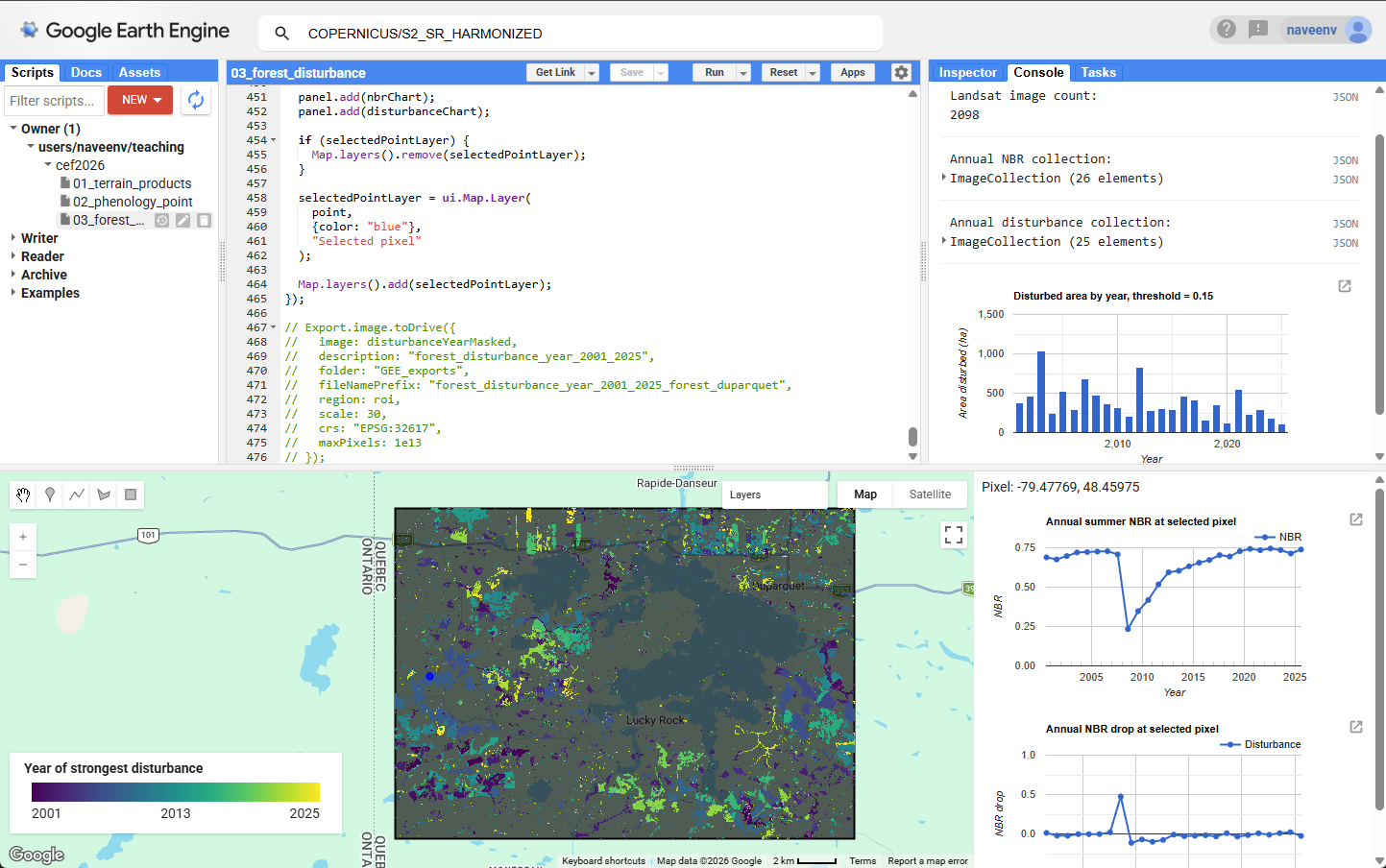
Forest disturbance year and pixel-level NBR time series

Example output showing the year of strongest forest disturbance and pixel-level Landsat NBR time series for the rectangular study area around Forêt Duparquet.

Visual check against reference layers¶

The disturbance map should be checked against independent information before interpreting detected disturbance as harvesting.

In the example below, the exported disturbance-year map is compared with existing forest inventory or disturbance reference layers. The comparison helps identify whether the detected disturbance patches have realistic shapes, locations, and years.

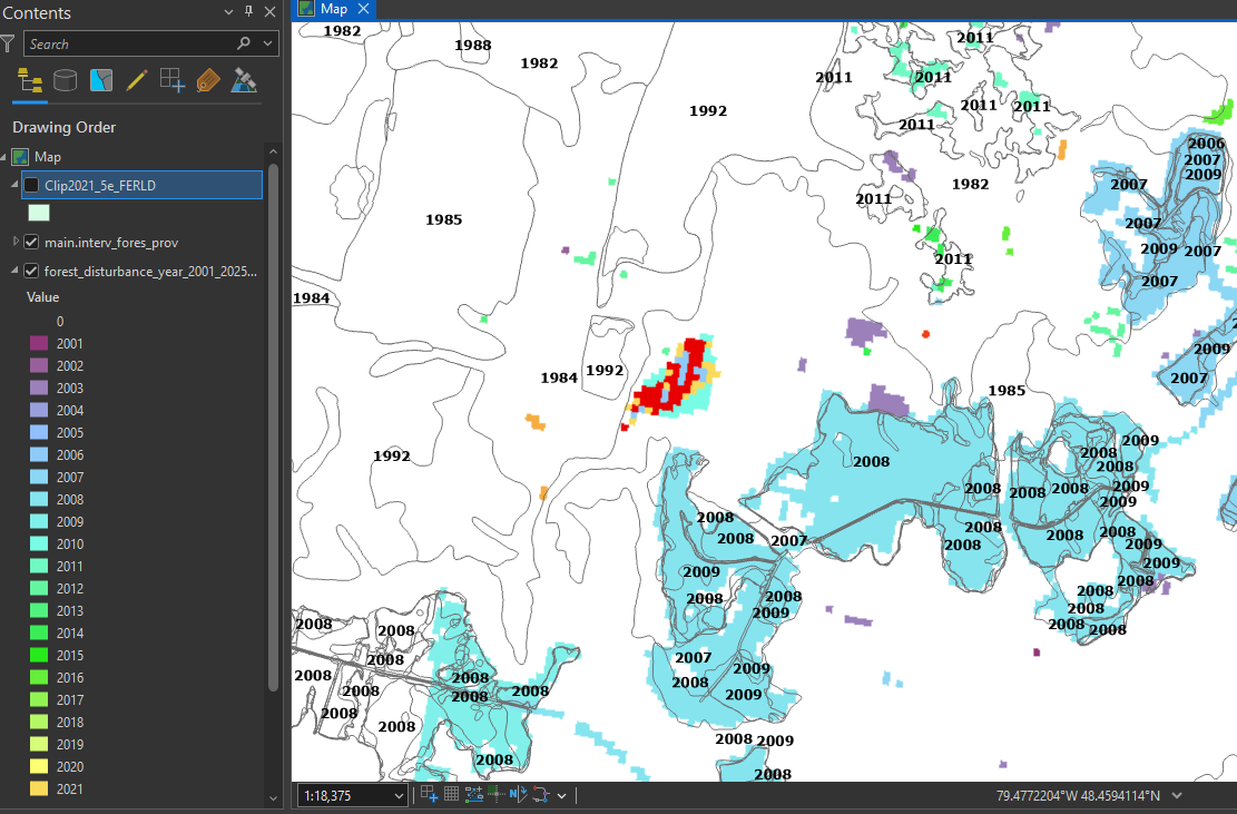
Visual comparison of mapped disturbance year with reference forest layers

Example 1. Visual check of the mapped year of maximum disturbance against reference forest layers.

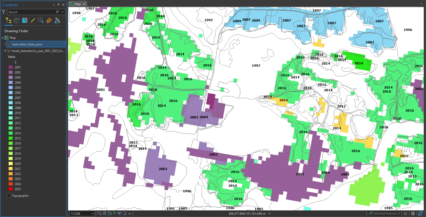
Second visual comparison of mapped disturbance year with reference layers

Example 2. Additional visual check in another part of the ROI.

This type of visual check can help answer three questions:

Do detected disturbance patches overlap known disturbance or management areas?
Do the mapped years appear reasonable compared with the reference information?
Are there obvious false detections near water, wetlands, roads, clouds, shadows, or mixed pixels?

A visual check is useful for interpretation, but it is not the same as a formal accuracy assessment. A formal validation would require independent reference samples and accuracy metrics such as a confusion matrix, user’s accuracy, producer’s accuracy, and overall accuracy.

Interpretation notes¶

High NBR values usually indicate dense, moist forest canopy.

Low NBR values may indicate harvested areas, burned areas, open vegetation, exposed soil, roads, wetlands, water, or other non-forest surfaces.

A sudden drop in NBR often indicates canopy disturbance. If the drop is large, spatially clustered, and forms patches with clear boundaries, it may represent harvesting or another strong disturbance event.

The threshold controls how much NBR drop is required before a pixel is mapped as disturbed. Lower thresholds detect more change but may include more noise. Higher thresholds produce cleaner maps but may miss subtle disturbance.

The disturbance year map shows the year with the strongest NBR drop for each pixel. It does not show every disturbance event, and it does not directly identify the cause of disturbance.

How to publish the app¶

After the app script runs correctly in the Earth Engine Code Editor:

Click Apps in the upper-right panel.
Click New App.
Select the cloud project, or choose Only me for restricted access.
Add an app name, for example: nbr-forest-disturbance.
Under App source code, choose either:
- Current contents of editor, or
- Repository script path
Click Publish.

The published app can be shared with users who want to explore the results without editing the code.

Questions¶

Click a stable forest pixel. How does its NBR change through time?
Click a disturbed pixel. In which year does the NBR drop sharply?
Does NBR recover after the disturbance? If yes, how quickly?
Does the mapped disturbance year match the pixel-level NBR drop?
How does the disturbance map change if the threshold is lowered from 0.20 to 0.10?
Which years show the largest disturbed area?
Do the detected disturbance patches have sharp, realistic boundaries?
Are there pixels that look like false detections?
What evidence would you need to confidently interpret a detected disturbance as harvesting?

Optional extension¶

Try changing the disturbance threshold.

var threshold = 0.15;

Then rerun the script and compare the disturbance year map and disturbed-area chart.

Check how the results change as you adjust the threshold:

Which pixels disappear when the threshold increases?
Do the remaining patches look more reliable?
Does the disturbed-area chart change substantially?